# openEO Cookbook
This is the openEO cookbook that you can refer to to get a first idea on how to solve problems with openEO in the three client languages Python, R and JavaScript. It describes how to implement simple use cases in a pragmatic way.
Please refer to the getting started guides for JavaScript, Python and R if you have never worked with one of the openEO client libraries before. This guide requires you to have a basic idea of how to establish a connection to a back-end and how to explore that back-end.
References
- openEO processes documentation
- openEO Hub (opens new window) to discover back-ends with available data and processes
- openEO Web Editor (opens new window) to visually build and execute processing workflows
# Chapter 1
In this chapter, we want to explore the different output formats that are possible with openEO. For that, we load and filter a collection (a datacube) of satellite data and calculate the temporal mean of that data. Different steps (e.g. a linear scaling) are done to prepare for the data to be output in one of the formats: Raster or text data.
Throughout this guide, code examples for all three client languages are given. Select your preferred language with the code switcher on the right-hand side to set all examples to that language.
# Connecting to a back-end
Click the link below to see how to connect to a back-end (via OpenID Connect). You can call the connection object con as it is done in all following code, to avoid confusion throughout the rest of the tutorials.
- Python
- R
- JavaScript
In R and JavaScript it is very useful to assign a graph-building helper object to a variable, to easily access all openEO processes and add them to the process graph that you will be building. These objects will be used throughout this guide. In Python, it also helps to import a helper object, even though we'll need it less often.
- Python
- R
- JavaScript
# import ProcessBuilder functions
from openeo.processes import ProcessBuilder
Note: Many functions in child processes (see below), are instances of this ProcessBuilder import.
# Input: load_collection
Before loading a collection, we need to find out the exact name of a collection we want to use (back-end-specific, see references at the top). We assign the spatial and temporal extent to variables, so that we can re-use them on other collections we might want to load. Let's look for a Sentinel 2 (preprocessed level 2A preferably) collection and load the green, red and a near-infrared band (bands 3, 4 and 8).
Collection and Band Names
The names of collections and bands differ between back-ends. So always check the collection description for the correct names. The differences might be subtle, e.g. B8 vs. B08.
We'll name our collection very explicitly cube_s2_b348 as to not get confused later on.
- Python
- R
- JavaScript
# make dictionary, containing bounding box
urk = {"west": 5.5661, "south": 52.6457, "east": 5.7298, "north": 52.7335}
# make list, containing the temporal interval
t = ["2021-04-26", "2021-04-30"]

# load first datacube
cube_s2_b348 = con.load_collection(
    "COPERNICUS/S2_SR",
    spatial_extent = urk,
    temporal_extent = t,
    bands = ["B3", "B4", "B8"]
)
# Filter Bands: filter_bands
To go through the desired output formats, we'll need one collection with three bands, and one collection with only one band. Here we use filter_bands, when of course we could also just define a separate collection via load_collection. As our input datacube already has the required three bands, we filter it for a single band to create an additional datacube with the same spatial and temporal extent, but with only one band (band 8).
We'll name this one cube_s2_b8 to distinguish it from the original cube_s2_b348.
- Python
- R
- JavaScript
# filter for band 8
cube_s2_b8 = cube_s2_b348.filter_bands(bands = ["B8"])
# Temporal Mean: reduce_dimension
As we don't want to download the raw collection of satellite data, we need to reduce that data somehow. That means, we want to get rid of one dimension. Let's say we calculate a mean over all timesteps, and then drop the temporal dimension (as it's empty then anyway, see explanation in the datacube guide). This can be done via reduce_dimension(). The function requires a reducer, in our case a mean process, and the dimension over which to reduce, given as a string ("t").
Child Processes
Here, we need to define a child process: A function that is called by (or passed to) another function, and then works on a subset of the datacube (somewhat similar to the concept of callbacks in JavaScript). In this case: We want reduce_dimension to use the mean function to average all timesteps of each pixel. Not any function can be used like this, it must be defined by openEO, of course.
All clients have more or less different specifics when defining a child process. As you can observe directly below, one way to define one is to define the function directly inside the parent process.
For a more clean way to define a child process, see the chapter below.
- Python
- R
- JavaScript
# reduce all timesteps
# mean_time() is a shortcut function
cube_s2_b8_red = cube_s2_b8.mean_time()

# alternatively, 'reduce_dimension' can be used
cube_s2_b8_red = cube_s2_b8.reduce_dimension(dimension="t", reducer="mean")

# additionally, reduce second collection
cube_s2_b348_red = cube_s2_b348.mean_time()
Note: In python, the child process can be a string.
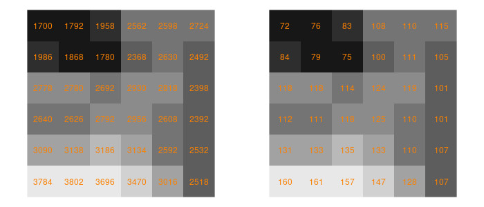
# Scale All Pixels Linearly: apply, linear_scale_range
To create a PNG output, we need to scale the satellite data we have down to the 8bit range of a PNG image. For this, the scale range of our imagery has to be known. For Sentinel 2 over urban and agricultural areas, we can use 6000 as a maximum.
We'll use the process linear_scale_range. It takes a number and the four borders of the intervals as input. Because it works on a number and not a datacube as all processes discussed so far, we need to nest the process into an apply, once again defining a child process. apply applies a unary process to all pixels of a datacube.
This time we'll also define our child processes externally, as to not get confused in too much code nesting.
- Python
- R
- JavaScript
# define child process, use ProcessBuilder
def scale_function(x: ProcessBuilder):
    return x.linear_scale_range(0, 6000, 0, 255)

# apply scale_function to all pixels
cube_s2_b348_red_lin = cube_s2_b348_red.apply(scale_function)
Resource: Refer to the Python client documentation (opens new window) to learn more about child processes in Python.
# Spatial Aggregation: aggregate_spatial
To look at text output formats we first need to "de-spatialize" our data. Or put another way: If we're interested in e.g. timeseries of various geometries, text output might be very interesting for us.
To aggregate over certain geometries, we use the process aggregate_spatial. It takes valid GeoJSON as input. We can pass a GeoJSON FeatureCollection in Python and JavaScript, but we need to introduce two packages in R, sf and geojsonsf, to convert the FeatureCollection string to a simple feature collection.
- Python
- R
- JavaScript
# polygons as (geojson) dict
polygons = { "type": "FeatureCollection", "features": [ { "type": "Feature", "properties": {}, "geometry": { "type": "Polygon", "coordinates": [ [ [ 5.636715888977051, 52.6807532675943 ], [ 5.629441738128662, 52.68157281641395 ], [ 5.633561611175536, 52.67787822078012 ], [ 5.636715888977051, 52.6807532675943 ] ] ] } }, { "type": "Feature", "properties": {}, "geometry": { "type": "Polygon", "coordinates": [ [ [ 5.622982978820801, 52.68595649102906 ], [ 5.6201934814453125, 52.68429152697491 ], [ 5.628776550292969, 52.683719180920846 ], [ 5.622982978820801, 52.68595649102906 ] ] ] } } ]}

# aggregate spatial
cube_s2_b8_agg = cube_s2_b8.aggregate_spatial(geometries = polygons, reducer = "mean")

# alternatively, the python client has a shortcut function for this special case
# cube_s2_b8_agg = cube_s2_b8.polygonal_mean_timeseries(polygon = polygons)
# Output: save_result
To get a result, we first need to create a save_result node, in which we state the desired output format and potential parameters, both dependent on the back-end you are connected to. The output formats and their parameters can e.g. be explored via the Web Editor along with available processes and collections.
We then proceed to send that job to the back-end, without executing it. Refer to the getting started guides on how to process results as batch or synchronous jobs. The way it is stated here allows us to log in to the Web Editor and look at, change, and execute the job from there.
# Raster Formats: GTiff, NetCDF
In the example, GeoTiff files are produced. Refer to the back-end for the available formats, options, and their correct naming. Check the PNG section for passing options.
Different from the creation of a PNG image, the raster format doesn't need scaling and the original datacube can be downloaded as is. However, we need to be careful with the dimensionality of the datacube: How a 4+ - dimensional datacube is handled when converted to a raster format is back-end dependent. That is why we made sure that our cube would only contain one additional dimension, apart from the spatial x and y.
- Python
- R
- JavaScript
# save using save_result, give format as string
res = cube_s2_b8_red.save_result(format = "GTiff")

# send job to back-end, do not execute
job = res.create_job(title = "temporal_mean_as_GTiff_py")
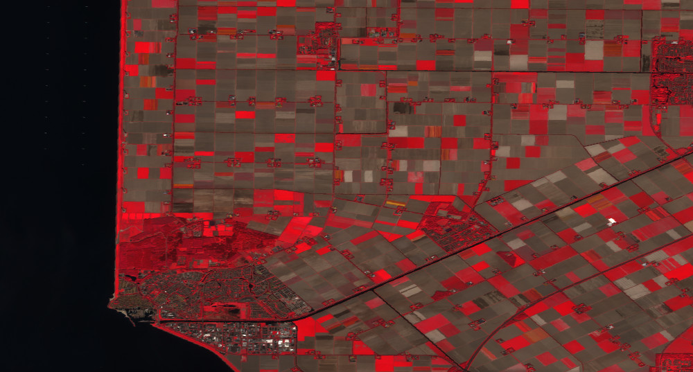
# Raster Formats: PNG
For a PNG output, we'll use the datacube with the bands 3, 4 and 8 (green, red and near-infrared) that we've been working on simultaneously with the datacube used above. As we have scaled the data down to 8bit using a linear scale, nothing stands in the way of downloading the data as PNG.
We want to produce a false-color composite highlighting the vegetation in red (as seen below the code). For that, we want to assign the infrared band (B8) to the red channel, the red band (B4) to the green channel and the green band (B3) to the blue channel. Some back-ends may offer to pass along this desired band order as it is shown below. Check with the back-end for available options.
Note
If no options can be passed, handling of the bands for PNG output is internal and should be documented by the back-end. You might also be able to tell how this is done by how your PNG looks: As explained in the datacube guide, the order of the bands dimension is defined when the values are loaded or altered (in our example: filter_bands). As we filter bands in the order "B3", "B4", "B8" vegetation might be highlighted in blue, given that the back-end uses the input order for the RGB channels.
The example below uses the PNG file format as defined by the Google Earth Engine back-end so the parameters red, green and blue may not be available on another back-end. Make sure to check the file format documentation for your back-end.
- Python
- R
- JavaScript
# save result cube as PNG
res = cube_s2_b348_red_lin.save_result(format = "PNG", options = {
        "red": "B8",
        "green": "B4",
        "blue": "B3"
      })

# send job to back-end
job = res.create_job(title = "temporal_mean_as_PNG_py")
In python, options are passed as a dictionary
# Text Formats: JSON, CSV
We can now save the timeseries in the aggregated datacube as e.g. JSON.
- Python
- R
- JavaScript
# save result cube as JSON
res = cube_s2_b8_agg.save_result(format = "JSON")

# send job to back-end
job = res.create_job(title = "timeseries_as_JSON_py")
# Output: Process as JSON
In some cases we want to export the JSON representation of a process we created. If you followed one of the examples above, then your end node is called res. If not, replace that with whatever you called your process end node.
- Python
- R
- JavaScript
process = res.to_json()

# if needed, write JSON to file, e.g.:
with open("./process.json", "w") as tfile:
    tfile.write(process)
# Chapter 2
In this second part of the cookbook, things are a bit less linear. We'll explore bandmath, masking and apply_* functionality, only that these steps are less interconnected than in the first chapter.
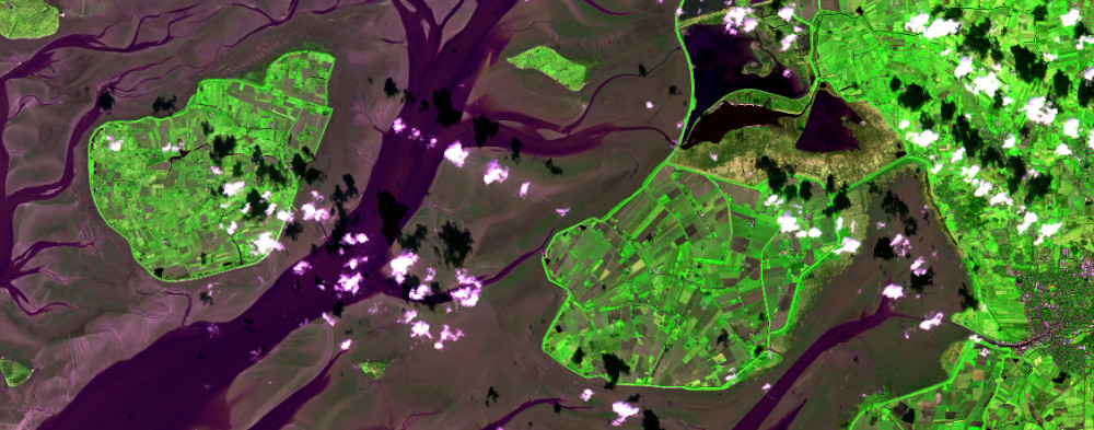
As usual we'll load a collection to work with (Sentinel 2, bands 2, 4, 8 and SCL). Let's call it cube_s2. We pre-select a time frame of which we know it only contains one Sentinel 2 scene, so that we're not bothered with multiple timesteps (the collection still contains a time dimension, but with only one timestep in it, so that it can be ignored). The extent has been chosen to provide results that are suitable to show the effect of the processes used, while being considerably small and thus fast to compute. If you want to minimize processing time you are of course free to use much smaller AOIs.
To be able to download and look at the results, refer to the output section of chapter 1. Most of the images in this tutorial were all downloaded as GTiff and plotted with R.
- Python
- R
- JavaScript
pellworm = {"west": 8.5464, "south": 54.4473, "east": 9.0724, "north": 54.5685}
t = ["2021-03-05", "2021-03-05"]

cube_s2 = con.load_collection(
    "SENTINEL2_L2A_SENTINELHUB",
    spatial_extent = pellworm,
    temporal_extent = t,
    bands = ["B02", "B04", "B08", "SCL"]
)
# Bandmath
Bandmath refers to computations that involve multiple bands, like indices (Normalized Difference Vegetation Index, Normalized Burn Ratio etc.).
In openEO, this goes along with using for example reduce_dimension over the bands dimension. In this process, a new pixel value is calculated from the values of different bands using a given formula (the actual bandmath), to then eliminate the bands dimension alltogether. If e.g. a cube contains a red and a nir band in its bands dimension and we reduce said dimension with a formula for the NDVI, that cube afterwards contains NDVI values, but no bands dimension anymore.
In the following we'll observe a thorough explanation of how to calculate an NDVI. That section covers different ways (depending on the client) to set up such a process in openEO. Afterwards, we'll see how an EVI is computed in a quicker, less thorough example.
# Example 1: NDVI
As mentioned above, bandmath is about reducing the bands dimension with a child process (a formula) that gives us the desired output. In chapter one, we already saw different ways of defining a child process: a) We learned how to use a simple mean to reduce the time dimension, and b) we saw how to access and use the openEO defined linear_scale_range function to scale all pixels linearly.
In this chapter, we'll reiterate these techniques and discuss some subtleties and alternatives. It is up to you to choose one that works best. Special to the NDVI is, given that it is the most common use case, that openEO has predefined processes that cover the math for us and only need to be given the correct input. There even is a function ndvi that masks all details and only takes a datacube and the bandnames as input. Further down we'll dig into what this ndvi process actually masks, how we can reproduce that manually, and thus how we could formulate other bandmath functions, apart from an NDVI.
By using the openEO defined ndvi function, calculating an NDVI becomes pretty straightforward. The process can detect the red and near-infrared band based on metadata and doesn't need bandname input (but band names can be passed to calculate other normalized differences). Also, by supplying the optional parameter target_band we can decide if we want to get a reduced cube with NDVI values and no bands dimension as result, or if we want to append the new NDVI band to the existing bands of our input cube. If we choose the latter, we only need to supply a name for that new NDVI band.
- Python
- R
- JavaScript
cube_s2_ndvi = cube_s2.ndvi()

# or name bands explicitly + append the result band to the existing cube
# cube_s2_ndvi_bands = cube_s2.ndvi(nir = "B08", red = "B04", target_band = "NDVI")
For the purpose of understanding, we'll stick with our NDVI example to explore different ways of defining bandmath in openEO. That gives you the knowledge to define other processes, not just NDVIs. The first method is available in all clients: Defining a function and passing it to a process, e.g. reduce_dimension. If available, other possibilities are discussed afterwards.
Important: Check Band Indices and Bandnames!
Be careful when handling the names or array indices of bands. While names differ across back-ends, indices can be mixed up easily when some other band is deleted from the input collection. Python and JavaScript have 0-based indices, R indices are 1-based. So double check which bands you're actually using.
- Python
- R
- JavaScript
# necessary imports
from openeo.processes import array_element, normalized_difference

# define an NDVI function
def ndvi_function(data):
    B04 = array_element(data, index = 1) # array_element takes either an index ..
    B08 = array_element(data, label = "B08") # or a label

    # ndvi = (B08 - B04) / (B08 + B04) # implement NDVI as formula ..
    ndvi = normalized_difference(B08, B04) # or use the openEO "normalized_difference" process

    return ndvi

# supply the defined function to a reduce_dimension process, set dimension = "bands"
cube_s2_ndvi = cube_s2.reduce_dimension(reducer = ndvi_function, dimension = "bands")
What we see above:
- access specific bands inside the child process:
array_element(supply data and index/label) - call openEO defined functions inside the child process by importing it:
from openeo.processes import normalized_difference - write math as formula inside the child process:
ndvi = (B08 - B04) / (B08 + B04)
The python client also holds a second possibility to do the above. It has a function band that does array_element and reduce_dimension(dimension = "bands") for us. When using it, we can type out the NDVI formula right in the script (since .band reduced the cube for us).
B04 = cube_s2.band("B04")
B08 = cube_s2.band("B08")

cube_s2_ndvi = (B08 - B04) / (B08 + B04) # type math formula
# Example 2: EVI
The formula for the Enhanced Vegetation Index is a bit more complicated than the NDVI one and contains constants. But we also don't necessarily need an openEO defined function and can concentrate on implementing a more complex formula. Here's the most efficient way to do this, per client.
- Python
- R
- JavaScript
# extract and reduce all bands via "band"
B02 = cube_s2.band("B02")
B04 = cube_s2.band("B04")
B08 = cube_s2.band("B08")

# write formula
cube_s2_evi = (2.5 * (B08 - B04)) / ((B08 + 6.0 * B04 - 7.5 * B02) + 1.0)
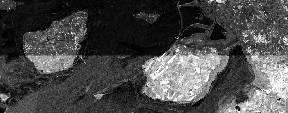
# Masks: mask
Masking generally refers to excluding (or replacing) specific areas from an image. This is usually done by providing a boolean mask that detemines which pixels to replace with a no-data value, and which to leave as they are. In the following we will consider two cases: a) Creating a mask from classification classes and b) creating a mask by thresholding an image.
# Mask Out Specific Values
In some cases we want to mask our data with other data. A common example is to mask out clouds, which optical satellites can not see through. Some Sentinel 2 collections provide the SCL classification band (see the table of classes at the bottom here (opens new window)), providing a representation coded into land cover classes. In this classification, vegetation is coded as 4 and non-vegetation as 5, while e.g. clouds are coded as 8 to 10.
In the following, we're building a mask using some logical operations as a child process while reducing the dimension bands. As explained at Example 1: NDVI this is done to be left with a cube that has no dimension bands. In R and JavaScript, we write a function filter_ that turns the values of the SCL band into 0s (for (non-) vegetation) and 1s (for all others), and ignores all other bands. During mask, all 1s (i.e. TRUE) pixels will be replaced, and as we don't define a replacement they will simply be set to null. In Python, in-line logical operations can be used.
- Python
- R
- JavaScript
# get classification band
SCL = cube_s2.band("SCL")

# we want to mask all other values, so NOT (4 OR 5)
cube_s2_mask = ~ ((SCL == 4) | (SCL == 5))

# masking
cube_s2_masked = cube_s2.mask(cube_s2_mask)
As with all functionality there are differences between back-ends. If this first example "Mask Out Specific Values" doesn't work for you, that could be because we are trying to apply a mask (a cube with dimensions x, y, t) to the input data (a cube with dimensions x, y, t, bands) and thus, cubes with different dimensionality. If you encounter such a problem, try applying the first mask to the NDVI cube (with dimensions x, y, t) as it is shown in the second example "Thresholds".
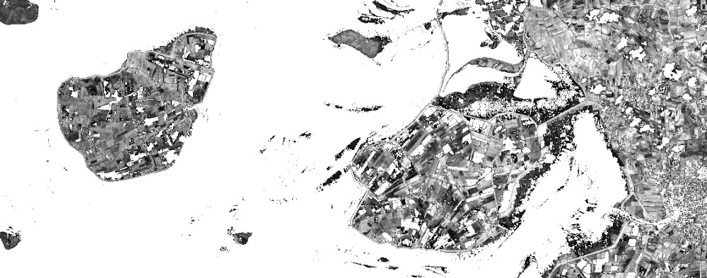
# Thresholds
In this scenario we want an image that contains all NDVI values above 0.3, and holds no-data values otherwise. This could be useful to have a look at the vegetation in the area, without being distracted by all other NDVI values. For this example we reuse the NDVI cube cube_s2_ndvi that was calculated in the NDVI bandmath-example, thus for this to work you must include said code into your script.
If you look closely, you'll notice that this time we're not using reduce_dimension to construct our masking cube (in contrast to Mask out Specific Values). In R and JavaScript we use apply instead, and in the python client no .band() is necessary anymore. This is because when we were masking using specific values of the band SCL, we were using the cube_s2 (with the bands B02, B04, B08 and SCL) as input. We then reduced the bands dimension by writing and passing the function filter_, which returned a cube that had no bands dimension anymore but 1s and 0s according to what we wanted to mask.
Here, we are making a mask out of the cube_s2_ndvi, a cube that had its band dimension already reduced when the NDVI was calculated. To turn its values into 1s and 0s, we only need to apply a threshold function. For this we utilize the openEO defined function lt ("less than"). As usual the clients expose different ways of getting to that function, one of which is shown below.
- Python
- R
- JavaScript
# create mask that is TRUE for NDVI < 0.3
ndvi_threshold = cube_s2_ndvi < 0.3

# apply mask to NDVI
cube_s2_ndvi_masked = cube_s2_ndvi.mask(ndvi_threshold)
# Pixel Operations: apply
As we remember from the datacube guide, unary processes take only the pixel itself into account when calculating new pixel values. We can implement that with the apply function and a child process that is in charge of modifying the pixel values. In our first example, that will be the square root. The openEO function is called sqrt. In the following we'll see how to pass it to the apply process.
- Python
- R
- JavaScript
# pass unary child process as string
cube_s2_sqrt = cube_s2.apply("sqrt")
Let's say we're not looking at optical but SAR imagery. Depending on the collection held by the back-end, this data could already be log-scaled. In case it isn't, we may want to transform our data from intensity values to db. This formula is a bit more complicated: 10 * log10(x). So we'll need a multiplication (by 10) and a log process (to the base 10).
Prior to applying the following code, we must load a collection containing SAR intensity data (e.g. Sentinel 1 GRD product).
- Python
- R
- JavaScript
# import the defined openEO process
from openeo.processes import log

# define a child process
def log_(x):
  return 10 * log(x, 10)

# supply that function to the "apply" call
cube_s1_log10 = cube_s1.apply(log_)
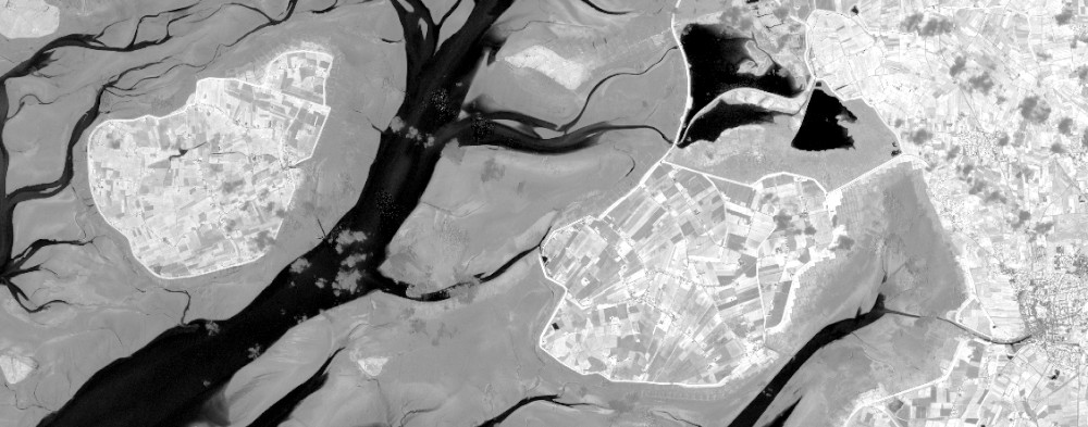
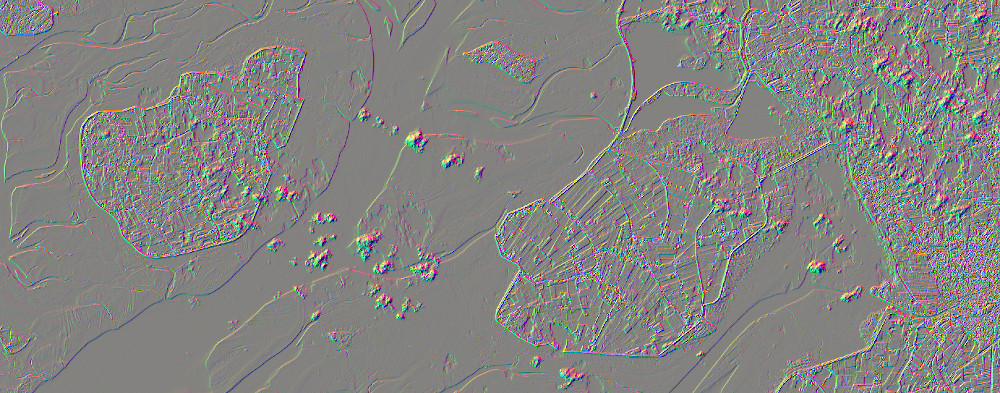
# Image Kernels: apply_kernel
The process apply_kernel takes an array of weights that is used as a moving window to calculate new pixel values. This is often used to smooth or sharped the image (e.g. Gaussian blur or highpass filter, respectively). Here, we show two Sobel edge detection kernels (both vertical and horizontal) and a highpass filter.
We'll only consider band 8 to shorten computation time.
- Python
- R
- JavaScript
cube_s2_b8 = cube_s2.filter_bands(["B08"])
Throughout all clients we can define the kernel as an array of arrays, of which the inner arrays represent lines (x) and the outer arrays columns (y). This means that by adding a line break after each inner array, a true representation of the kernel can be created (see highpass in Python or JavaScript tab).
The parameters factor and border are not needed here and are left out to fall back to default. factor (default 1) is multiplied with each pixel after the focal operation, while border (default 0) defines how overlaps between the kernel and the image borders are handled (should pixel values be mirrored, replicated or simply set to 0?, see apply_kernel).
- Python
- R
- JavaScript
# we can pass a kernel as an array of arrays
sobel_vertical = [[1, 2, 1], [0, 0, 0], [-1, -2, -1]] # e.g. 3x3 edge detection
sobel_horizontal = [[1, 0, -1], [2, 0, -2], [1, 0, -1]]

highpass = [ # or 5x5 highpass filter
  [-1, -1, -1, -1, -1],
  [-1, -1, -1, -1, -1],
  [-1, -1, 24, -1, -1],
  [-1, -1, -1, -1, -1],
  [-1, -1, -1, -1, -1]
]

# apply to cube
cube_s2_highpass = cube_s2_b8.apply_kernel(highpass)
# Endnote
You have feedback or noticed an error? Feel free to open an issue in the github repository (opens new window) or use the other communication channels (opens new window)