# R Client

# Useful links

Documentation (opens new window)
Vignettes (opens new window)
Code Repository (opens new window)
for function documentation, use R's ? function or see the online documentation (opens new window)

# Installation

Before you install the R client module into your R environment, please make sure that you have at least R version 3.6. Older versions might also work, but were not tested.

Stable releases can be installed from CRAN:

install.packages("openeo")

Installing the development version

If you want to install the development version, you can install from GitHub. It may contain more features, but may also be unstable.

You need to have the package 'devtools' installed. If it is not installed use install.packages("devtools").

Now you can use install_github from the devtools package to install the development version:

devtools::install_github(repo="Open-EO/openeo-r-client", dependencies=TRUE, ref="develop")

If this gives you an error, something went wrong with the installation so please check the requirements again.

If you have troubles installing the package, feel free to contact us or leave an issue at the GitHub project (opens new window).

Now that the installation was successfully finished, we can load the package and connect to openEO compliant back-ends. In the following chapters we quickly walk through the main features of the R client.

# Exploring a back-end

If you do not know an openEO back-end that you want to connect to yet, you can have a look at the openEO Hub (opens new window), to find all known back-ends with information on their capabilities.

For this tutorial we will use the openEO instance of Google Earth Engine, which is available at https://earthengine.openeo.org. Note that the code snippets in this guide work the same way for the other back-ends listed in the openEO Hub. Just the collection identifier and band names might differ.

First we need to establish a connection to the back-end.

library(openeo)
gee = connect(host = "https://earthengine.openeo.org")

The object stored as variable gee is a connection and resembles the OpenEOClient - an object, that bundles all information and functions to interact with the openEO back-end. It can be used explicitly in all of the functions to determine which connection has to be used (usually parameter con). If only one connection is active, then you can omit the parameter, because the last active connection is always stored in a package environment and used if no specific connection was present (see ?active_connection in the package documentation).

The capabilities of the back-end and the collections are generally publicly available, unless the data collections are proprietary and licensing issues prevent the back-end provider from publishing the collection. For the publicly available information you do not need to have an account on the back-end for reading them.

# Collections

Collections represent the basic data the back-end provides (e.g. Sentinel 1 collection) and are therefore often used as input data for job executions (more info on collections). With the following code snippet you can get all available collection names and their description. The collection list and its entries have their own implementations of the print function. The collection list object is coerced into a data.frame only for printing purposes and the collection for the collection some key information are printed.

To get the collection list can be indexed by the collections ID to get the more details about the overview information. With the describe_collection function you can get an even more detailed information about the collection.

# get the collection list
collections = list_collections()

# print an overview of the available collections (printed as data.frame or tibble)
print(collections)

# to print more of the reduced overview metadata
print(collections$`COPERNICUS/S2`)

# Dictionary of the full metadata of the "COPERNICUS/S2" collection (dict)
s2 = describe_collection("COPERNICUS/S2") # or use the collection entry from the list, e.g. collections$`COPERNICUS/S2`
print(s2)

In general all metadata objects are based on lists, so you can use str() to get the structure of the list and address fields by the $ operator.

TIP

If the package is used with RStudio the metadata can also be nicely rendered as a web page in the viewer panel by running collection_viewer(x="COPERNICUS/S2").

# Processes

Processes in openEO are tasks that can be applied to (EO) data. The input of a process might be the output of another process, so that several connected processes form a new (user-defined) process itself. Therefore, a process resembles the smallest unit of task descriptions in openEO (more details on processes). The following code snippet shows how to get the available processes.

# List of available openEO processes with full metadata
processes = list_processes()

# List of available openEO processes by identifiers (string)
print(names(processes))

# print metadata of the process with ID "load_collection"
print(processes$load_collection)

The list_processes() method returns a list of process metadata objects that the back-end provides. Each process list entry is a more complex list object (called 'ProcessInfo') and contains the process identifier and additional metadata about the process, such as expected arguments and return types.

TIP

As for the collection, processes can also be rendered as a web page in the viewer panel, if RStudio is used. In order to open the viewer use process_viewer() with either a particular process (process_viewer("load_collection")) or you can pass on all processes (process_viewer(processes)). When all processes are chosen, there is also a search bar and a category tree.

For other graphical overviews of the openEO processes, there is an online documentation for general process descriptions and the openEO Hub (opens new window) for back-end specific process descriptions.

# Authentication

In the code snippets above, authentication is usually not necessary, since we only fetch general information about the back-end. To run your own jobs at the back-end or to access job results, you need to authenticate at the back-end.

Depending on the back-end, there might be two different approaches to authenticate. You need to inform yourself at your back-end provider of choice, which authentication approach you have to carry out and how to obtain login credentials for yourself and your 'openeo' installation in R.

You can also have a look at the openEO Hub (opens new window) to see the available authentication types of the back-ends. For Google Earth Engine, only Basic Authentication is supported at the moment.

Recommendation

The Google Earth Engine implementation for openEO only supports Basic authentication, but generally the preferred authentication method is OpenID Connect due to better security mechanisms implemented in the OpenID Connect protocol.

# Basic Authentication

The Basic authentication method is a common way of authenticate HTTP requests given username and password.

The following code snippet shows how to log in via Basic authentication:

login(login_type="basic",
      user="user",
      password="password")

TIP

You can get username and password here: https://github.com/Open-EO/openeo-earthengine-driver#demo (opens new window)

After successfully calling the login method with the "basic" login type, you are logged into the back-end with your account. This means, that every call that comes after that via the connection variable is executed by your user account.

# OpenID Connect Authentication

WARNING

For Google Earth Engine, only Basic Authentication is supported at the moment.

The OIDC (OpenID Connect (opens new window)) authentication can be used to authenticate via an external service.

The following code snippet shows how to log in via OIDC authentication if the back-end supports the simplified authentication method:

login()

The following code snippet shows how to log in via OIDC authentication if the simplified authentication method doesn't work and you need to provide a client ID and secret:

# get supported OIDC providers which the back-end supports
oidc_providers = list_oidc_providers()

login(provider = oidc_providers$some_provider,
      config = list(
        client_id= "...",
        secret = "..."))

Calling this method opens your system web browser, with which you can authenticate yourself on the back-end authentication system. After that the website will give you the instructions to go back to the R client, where your connection has logged your account in. This means, that every call that comes after that via the connection variable is executed by your user account.

# Creating a (user-defined) process

Now that we know how to discover the back-end and how to authenticate, lets continue by creating a new batch job to process some data.

First we need to create a process builder object that carries all the available predefined openEO processes of the connected back-end as attached R functions with the parameters stated in the process metadata.

p = processes()

The functions of the builder return process nodes, which represent a particular result in the workflow. As one of the first steps we need to select the source data collection.

datacube = p$load_collection(
  id = "COPERNICUS/S1_GRD",
  spatial_extent=list(west = 16.06, south = 48.06, east = 16.65, north = 48.35),
  temporal_extent=c("2017-03-01", "2017-04-01"),
  bands=c("VV", "VH")
)

This results in a process node that represents a datacube and contains the "COPERNICUS/S1_GRD" data restricted to the given spatial extent, the given temporal extent and the given bands .

Sample Data Retrieval

In order to get a better understanding about the processing mechanisms and the data structures used in openEO Platform, it helps to check the actual data from time to time. The function get_sample (opens new window) aids the user in downloading data for a very small spatial extent. It is automatically loaded into R so that you can directly inspect it with stars. Read the vignette on "Sample Data Retrieval (opens new window)" for more details.

Having the input data ready, we want to apply a process on the datacube. Therefore, we can call the process directly on the datacube object, which then returns a datacube with the process applied.

min_reducer = function(data,context) { 
  return(p$min(data = data))
}

reduced = p$reduce_dimension(data = datacube, reducer = min_reducer, dimension="t")

The datacube is now reduced by the time dimension named t, by taking the minimum value of the timeseries values. Now the datacube has no time dimension left. Other so called "reducer" processes exist, e.g. for computing maximum and mean values.

Note

Everything applied to the datacube at this point is neither executed locally on your machine nor executed on the back-end. It just defines the input data and process chain the back-end needs to apply when it sends the datacube to the back-end and executes it there. How this can be done is the topic of the next chapter.

After applying all processes you want to execute, we need to tell the back-end to export the datacube, for example as GeoTiff:

formats = list_file_formats()

result = p$save_result(data = reduced, format = formats$output$`GTIFF-ZIP`)

The first line retrieves the back-ends offered input and output formats. The second line creates the result node, which stores the data as a zipped GeoTiff.

# Batch Job Management

After you have finished working on your (user-defined) process, we can now send it to the back-end and start the execution. In openEO, an execution of a (user-defined) process is called a (batch) job. Therefore, we need to create a job at the back-end using our datacube, giving it the title Example Title.

job = create_job(graph=result,title = "Example Title")

The create_job method sends all necessary information to the back-end and creates a new job, which gets returned. After this, the job is just created, but has not started the execution at the back-end yet. It needs to be queued for processing explicitly:

start_job(job = job)

After the job was executed, status updates can be fetched by using the list_jobs() function. This function returns a list of job descriptions, which can be indexed with the jobs ID to limit the search results. But remember that only list_jobs() refreshes this list. So, to monitor a job you have to iteratively call the job (describe_job()) or the job list list_jobs().

jobs = list_jobs()
jobs # printed as a tibble or data.frame, but the object is a list

# or use the job id (in this example 'cZ2ND0Z5nhBFNQFq') as index to get a particular job overview
jobs$cZ2ND0Z5nhBFNQFq

# alternatively request detailed information about the job
describe_job(job = job)

When the job is finished, calling download_results() will download the results of a job. Using list_results() will return an overview about the created files and their download link or it states the error message, in case of an error.

# list the processed results
list_results(job = job)

# download all the files into a folder on the file system
download_results(job = job, folder = "/some/folder/on/filesystem")

Note

The printing behavior and the actual data structure might differ!

Now you know the general workflow of job executions.

# Full Example

In this chapter we will show a full example of an earth observation use case using the R client and the Google Earth Engine back-end. Instead of batch job processing, we compute the image synchronously. Synchronous processing means the result is directly returned in the response, which usually works only for smaller amounts of data.

Use Case

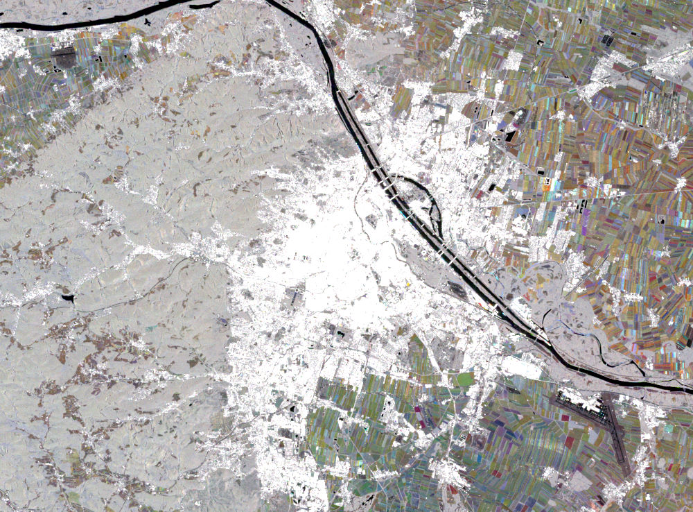
We want to produce a monthly RGB composite of Sentinel 1 backscatter data over the area of Vienna, Austria for three months in 2017. This can be used for classification and crop monitoring.

In the following code example, we use inline code comments to describe what we are doing.

WARNING

The username and password in the example above work at the time of writing, but may be invalid at the time you read this. Please contact us for credentials.

library(openeo)
library(tibble)

user = "group7"
pwd = "test123"

# connect  to the back-end and login either via explicit call of login, or use your credentials in the connect function
gee = connect(host = "https://earthengine.openeo.org",user = user,password = pwd,login_type = "basic")

# get the process collection to use the predefined processes of the back-end
p = processes()

# get the collection list to get easier access to the collection ids, via auto completion
collections = list_collections()

# get the formats
formats = list_file_formats()

# load the initial data collection and limit the amount of data loaded
# note: for the collection id and later the format you can also use the its character value
data = p$load_collection(id = collections$`COPERNICUS/S1_GRD`,
                         spatial_extent = list(west=16.06, 
                                               south=48.06,
                                               east=16.65,
                                               north=48.35),
                         temporal_extent = c("2017-03-01", "2017-06-01"),
                         bands = c("VV"))

# create three monthly sub data sets, which will be merged back into a single data cube later
march = p$filter_temporal(data = data,
                          extent = c("2017-03-01", "2017-04-01"))

april = p$filter_temporal(data = data,
                          extent = c("2017-04-01", "2017-05-01"))

may = p$filter_temporal(data = data,
                        extent = c("2017-05-01", "2017-06-01"))

# The aggregation function for the following temporal reducer
agg_fun_mean = function(data, context) {
  mean(data)
}

march_reduced = p$reduce_dimension(data = march,
                                   reducer = agg_fun_mean,
                                   dimension = "t")

april_reduced = p$reduce_dimension(data = april,
                                   reducer = agg_fun_mean,
                                   dimension = "t")

may_reduced = p$reduce_dimension(data = may,
                                 reducer = agg_fun_mean,
                                 dimension = "t")

# Each band is currently called VV. We need to rename at least the label of one dimension, 
# because otherwise identity of the data cubes is assumed. The bands dimension consists 
# only of one label, so we can rename this to be able to merge those data cubes.
march_renamed = p$rename_labels(data = march_reduced,
                                dimension = "bands",
                                target = c("R"),
                                source = c("VV"))

april_renamed = p$rename_labels(data = april_reduced,
                                dimension = "bands",
                                target = c("G"),
                                source = c("VV"))

may_renamed = p$rename_labels(data = may_reduced,
                              dimension = "bands",
                              target = c("B"),
                              source = c("VV"))

# combine the individual data cubes into one
# this is done one by one, since the dimensionalities have to match between each of the data cubes
merge_1 = p$merge_cubes(cube1 = march_renamed,cube2 = april_renamed)
merge_2 = p$merge_cubes(cube1 = merge_1, cube2 = may_renamed)

# rescale the the back scatter measurements into 8Bit integer to view the results as PNG
rescaled = p$apply(data = merge_2,
        process = function(data,context) {
          p$linear_scale_range(x=data, inputMin = -20,inputMax = -5, outputMin = 0, outputMax = 255)
        })

# export shall be format PNG
# look at the format description
formats$output$PNG

# store the results using the format and set the create options
result = p$save_result(data = rescaled,format = formats$output$PNG, options = list(red="R",green="G",blue="B"))

# create a job
job = create_job(graph = result, title = "S1 Example R", description = "Getting Started example on openeo.org for R-client")

# then start the processing of the job and turn on logging (messages that are captured on the back-end during the process execution)
start_job(job = job, log = TRUE)

Now the resulting PNG file of the RGB backscatter composite is stored as a PNG file in the current working directory. It looks like this:

RGB composite

TIP

The source code (opens new window) of the example can also be found on the R client repository on Github.

# User Defined Functions

If your use case can not be accomplished with the default processes of openEO, you can define a user defined function.

In general the processing workflow works by uploading the Python or R script into the users file directory on the back-end and reference the script via its URL or by its relational name (e.g. /scripts/script1.R) in the function run_udf. The latter function is a predefined openEO process that the back-end might provide, if UDFs are supported.

Find out more about UDFs in the respective Python UDF (opens new window) and R UDF (opens new window) repositories with their documentation and examples.