# Datacubes
# What are Datacubes?
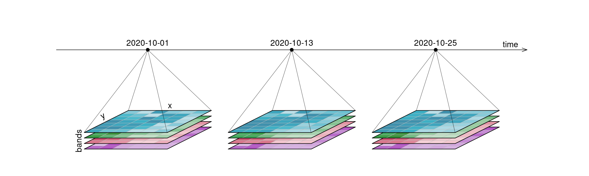
Data is represented as datacubes in openEO, which are multi-dimensional arrays with additional information about their dimensionality. Datacubes can provide a nice and tidy interface for spatiotemporal data as well as for the operations you may want to execute on them. As they are arrays, it might be easiest to look at raster data as an example, even though datacubes can hold vector data as well. Our example data however consists of a 6x7 raster with 4 bands [blue, green, red, near-infrared] and 3 timesteps [2020-10-01, 2020-10-13, 2020-10-25], displayed here in an orderly, timeseries-like manner:
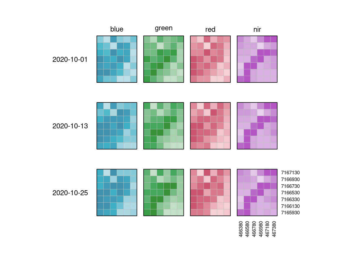
It is important to understand that datacubes are designed to make things easier for us, and are not literally a cube, meaning that the above plot is just as good a representation as any other. That is why we can switch the dimensions around and display them in whatever way we want, including the view below:
A vector datacube on the other hand could look like this:
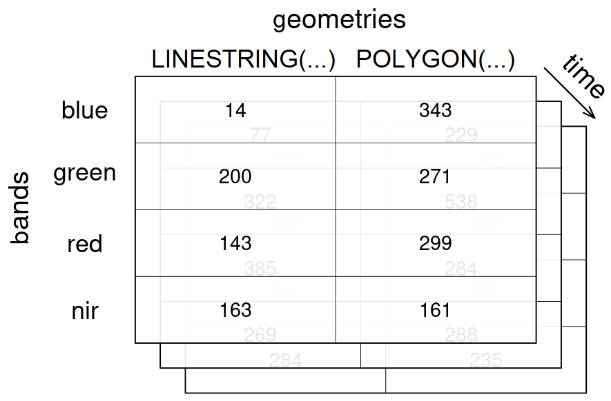
geometries dimension, along with 3 timesteps for the temporal dimension time and 4 bands in the bands dimension.Vector datacubes (opens new window) and raster datacubes are common cases of datacubes in the EO domain.
A raster datacube has at least two spatial dimensions (usually named x and y) and a vector datacube has at least one geometry dimension (usually named geometry).
The purpose of these distinctions is simply to make it easier to describe "special" cases of datacubes, but you can also define other types such as a temporal datacube that has at least one temporal dimension (usually named t).
The following additional information are usually available for datacubes:
All these information are usually provided through the datacube metadata.
# Dimensions
A dimension refers to a certain axis of a datacube. This includes all variables (e.g. bands), which are represented as dimensions. Our exemplary raster datacube has the spatial dimensions x and y, and the temporal dimension t. Furthermore, it has a bands dimension, extending into the realm of what kind of information is contained in the cube.
The following properties are usually available for dimensions:
- name
- type (potential types include: spatial (raster or vector data), temporal and other data such as bands)
- axis (for spatial dimensions) / number
- labels (usually exposed through textual or numerical representations, in the metadata as nominal values and/or extents)
- reference system / projection
- resolution / step size
- unit for the labels (either explicitly specified or implicitly provided by the reference system)
- additional information specific to the dimension type (e.g. the geometry types for a dimension containing geometries)
All these information are usually provided through the datacube metadata.
Here is an overview of the dimensions contained in our example raster datacube above:
| # | name | type | labels | resolution | reference system |
|---|---|---|---|---|---|
| 1 | x | spatial | 466380, 466580, 466780, 466980, 467180, 467380 | 200m | EPSG:32627 (opens new window) |
| 2 | y | spatial | 7167130, 7166930, 7166730, 7166530, 7166330, 7166130, 7165930 | 200m | EPSG:32627 (opens new window) |
| 3 | bands | bands | blue, green, red, nir | 4 bands | - |
| 4 | t | temporal | 2020-10-01, 2020-10-13, 2020-10-25 | 12 days | Gregorian calendar / UTC |
Dimension labels are usually either numerical or text (also known as "strings"), which also includes textual representations of timestamps or geometries for example. For example, temporal labels are usually encoded as ISO 8601 (opens new window) compatible dates and/or times and similarly geometries can be encoded as Well-known Text (WKT) (opens new window) or be represented by their IDs.
Dimensions with a natural/inherent order (usually all temporal and spatial raster dimensions) are always sorted. Dimensions without inherent order (usually bands), retain the order in which they have been defined in metadata or processes (e.g. through filter_bands (opens new window)), with new labels simply being appended to the existing labels.
A geometry dimension is not included in the example raster datacube above and it is not used in the following examples, but to show how a vector dimension with two polygons could look like:
| name | type | labels | reference system |
|---|---|---|---|
geometry | vector | POLYGON((-122.4 37.6,-122.35 37.6,-122.35 37.64,-122.4 37.64,-122.4 37.6)), POLYGON((-122.51 37.5,-122.48 37.5,-122.48 37.52,-122.51 37.52,-122.51 37.5)) | EPSG:4326 (opens new window) |
A dimension with geometries can consist of points, linestrings, polygons, multi points, multi linestrings, or multi polygons.
It is not possible to mix geometry types, but the single geometry type with their corresponding multi type can be combined in a dimension (e.g. points and multi points).
Empty geometries (such as GeoJSON features with a null geometry or GeoJSON geometries with an empty coordinates array) are allowed and can sometimes also be the result of certain vector operations such as a negative buffer.
# Applying Processes on Dimensions
Some processes are typically applied "along a dimension". You can imagine said dimension as an arrow and whatever is happening as a parallel process to that arrow. It simply means: "we focus on this dimension right now".
# Resolution
The resolution of a dimension gives information about what interval lies between observations. This is most obvious with the temporal resolution, where the intervals depict how often observations were made. Spatial resolution gives information about the pixel spacing, meaning how many 'real world meters' are contained in a pixel. The number of bands and their wavelength intervals give information about the spectral resolution.
# Coordinate Reference System as a Dimension
In the example above, x and y dimension values have a unique relationship to world coordinates through their coordinate reference system (CRS). This implies that a single coordinate reference system is associated with these x and y dimensions. If we want to create a data cube from multiple tiles spanning different coordinate reference systems (e.g. Sentinel-2: different UTM zones), we would have to resample/warp those to a single coordinate reference system. In many cases, this is wanted because we want to be able to look at the result, meaning it is available in a single coordinate reference system.
Resampling is however costly, involves (some) data loss, and is in general not reversible. Suppose that we want to work only on the spectral and temporal dimensions of a data cube, and do not want to do any resampling. In that case, one could create one data cube for each coordinate reference system. An alternative would be to create one single data cube containing all tiles that has an additional dimension with the coordinate reference system. In that data cube, x and y no longer point to a unique world coordinate, because identical x and y coordinate pairs occur in each UTM zone. Now, only the combination (x, y, crs) has a unique relationship to the world coordinates.
On such a crs-dimensioned data cube, several operations make perfect sense, such as apply or reduce_dimension on spectral and/or temporal dimensions. A simple reduction over the crs dimension, using sum or mean would typically not make sense. The "reduction" (removal) of the crs dimension that is meaningful involves the resampling/warping of all sub-cubes for the crs dimension to a single, common target coordinate reference system.
# Values in a datacube
openEO datacubes contain scalar values (e.g. strings, numbers or boolean values), with all other associated attributes stored in dimensions (e.g. coordinates or timestamps). Attributes such as the CRS or the sensor can also be turned into dimensions. Be advised that in such a case, the uniqueness of pixel coordinates may be affected. When usually, (x, y) refers to a unique location, that changes to (x, y, CRS) when (x, y) values are reused in other coordinate reference systems (e.g. two neighboring UTM zones).
Be Careful with Data Types
As stated above, datacubes only contain scalar values. However, implementations may differ in their ability to handle or convert them. Implementations may also not allow mixing data types in a datacube. For example, returning a boolean value for a reducer on a numerical datacube may result in an error on some back-ends. The recommendation is to not change the data type of values in a datacube unless the back-end supports it explicitly.
Data cube values can be sampled in two different ways. The values are either area or point samples.
- Area sampling aggregates measurements over defined regions, i.e. the grid cells for raster data or polygons/lines for vector data.
- Point sampling collects data at specific locations, providing detailed information for specific points.
# Processes on Datacubes
In the following part, the basic processes for manipulating datacubes are introduced.
# Filter
When filtering data (e.g. filter_spatial (opens new window), filter_temporal (opens new window), filter_bands (opens new window)), only the data that satisfies a condition is returned. For example, this condition could be a timestamp or interval, (a set of) coordinates, or specific bands. By applying filtering the datacube becomes smaller, according to the selected data.
Simplified
filter([🌽, 🥔, 🐷], isVegetarian) => [🌽, 🥔]
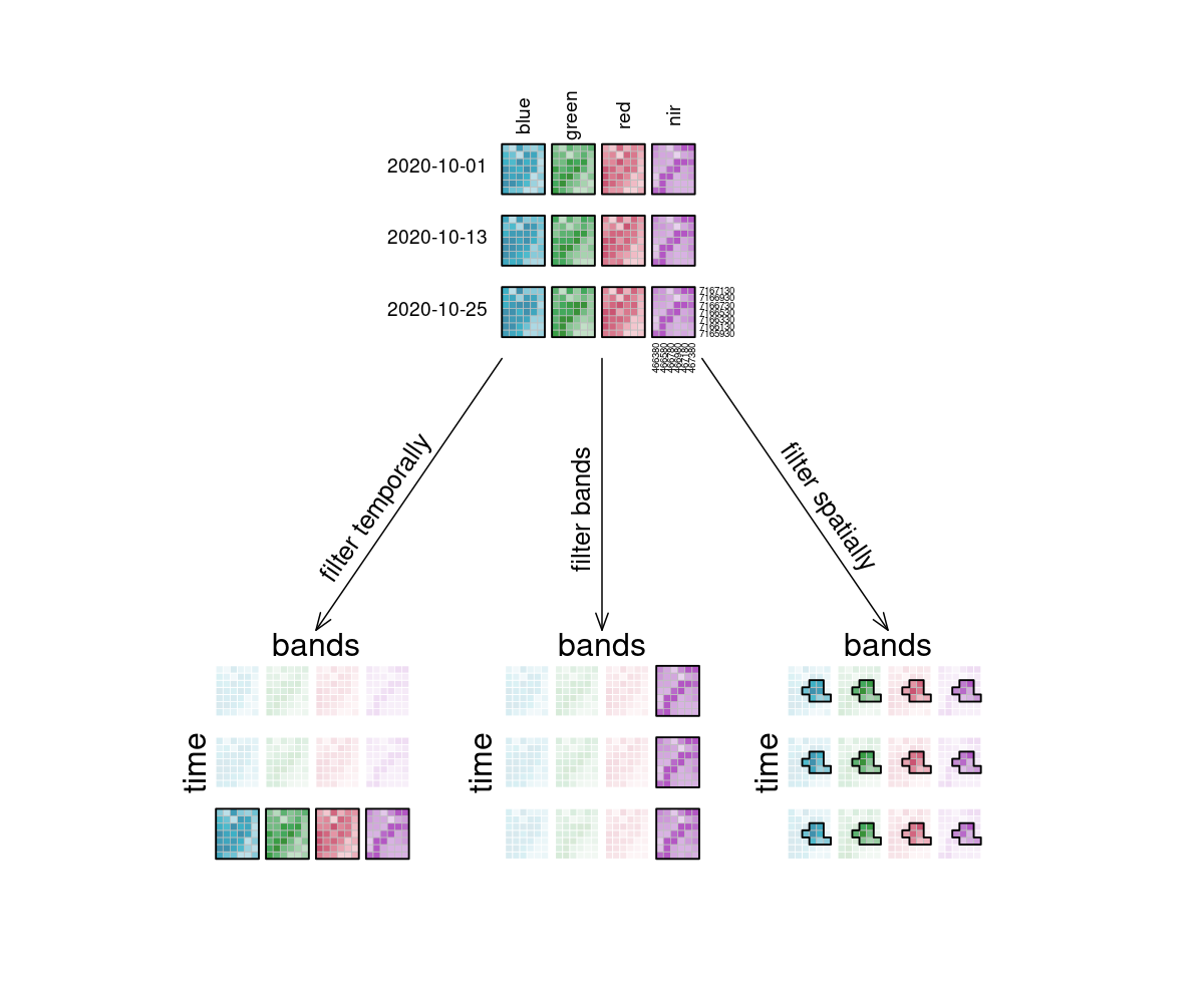
In the image, the example datacube can be seen at the top with labeled dimensions. The filtering techniques are displayed separately below. On the left, the datacube is filtered temporally with the interval ["2020-10-15", "2020-10-27"]. The result is a cube with only the rasters for the timestep that lies within that interval ("2020-10-25") and unchanged bands and spatial dimensions. Likewise, the original cube is filtered for a specific band ["nir"] in the middle and a specific spatial region [Polygon(...)] on the right.
# Apply
The apply* functions (e.g. apply (opens new window), apply_neighborhood (opens new window), apply_dimension (opens new window)) employ a process on the datacube that calculates new pixel values for each pixel, based on n other pixels. Please note that several programming languages use the name map instead of apply, but they describe the same type of function.
Simplified
apply([🌽, 🥔, 🐷], cook) => [🍿, 🍟, 🍖]
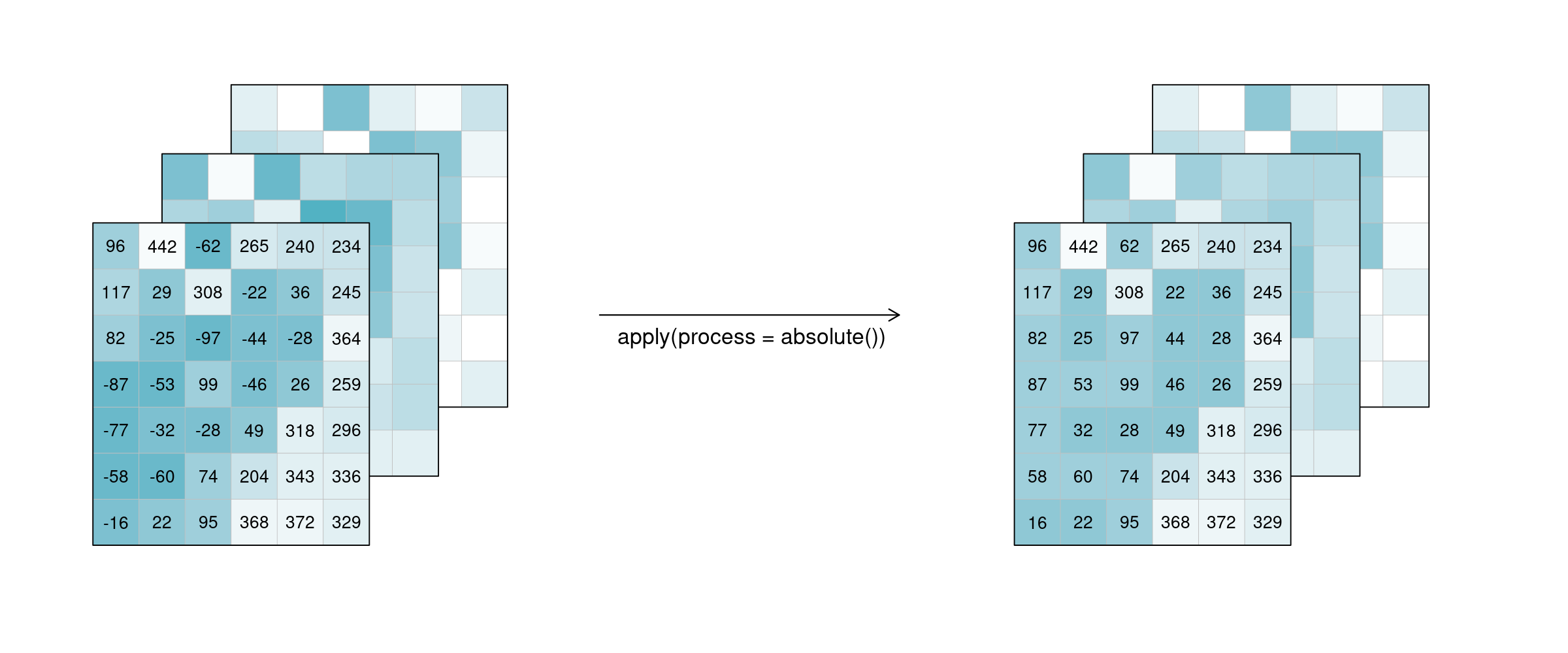
For the case n = 1 this is called a unary function and means that only the pixel itself is considered when calculating the new pixel value. A prominent example is the absolute() function, calculating the absolute value of the input pixel value.
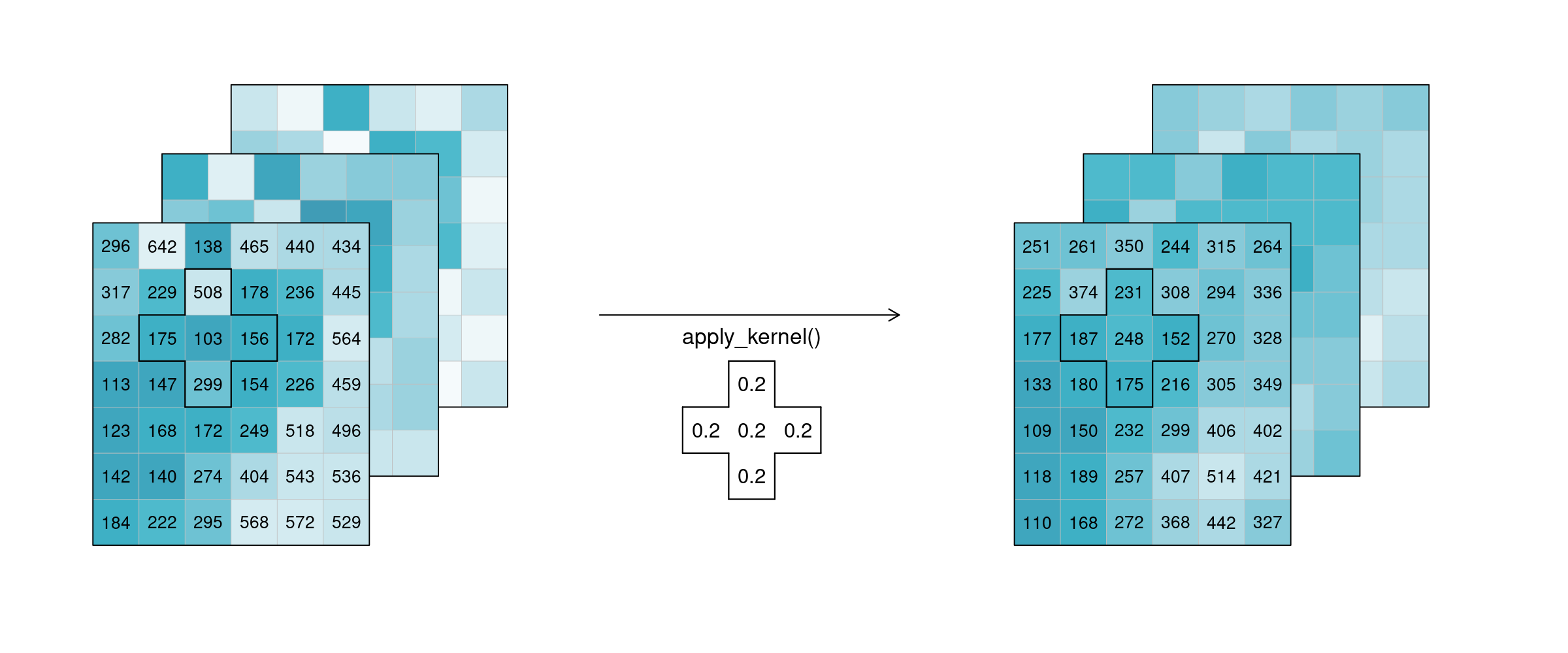
If n is larger than 1, the function is called n-ary. In practice, this means that the pixel neighbourhood is taken into account to calculate the new pixel value. Such neighbourhoods can be of spatial and/or temporal nature. A spatial function works on a kernel that weights the surrounding pixels (e.g. smoothing values with nearby observations), a temporal function works on a time series at a certain pixel location (e.g. smoothing values over time). Combinations of types to n-dimensional neighbourhoods are also possible.
In the example below, an example weighted kernel (shown in the middle) is applied to the cube (via apply_kernel (opens new window)). To avoid edge effects (affecting pixels on the edge of the image with less neighbours), a padding has been added in the background.
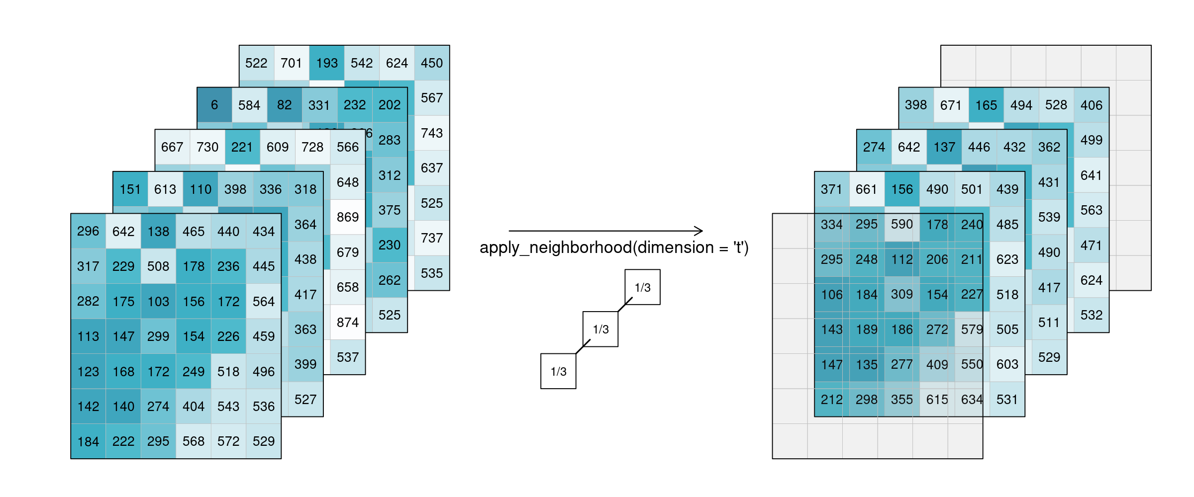
Of course this also works for temporal neighbourhoods (timeseries), considering neighbours before and after a pixel. To be able to show the effect, two timesteps were added in this example figure. A moving average of window size 3 is then applied, meaning that for each pixel the average is calculated out of the previous, the next, and the timestep in question (tn-1, tn and tn+1). No padding was added which is why we observe edge effects (NA values are returned for t1 and t5, because their temporal neighbourhood is missing input timesteps).
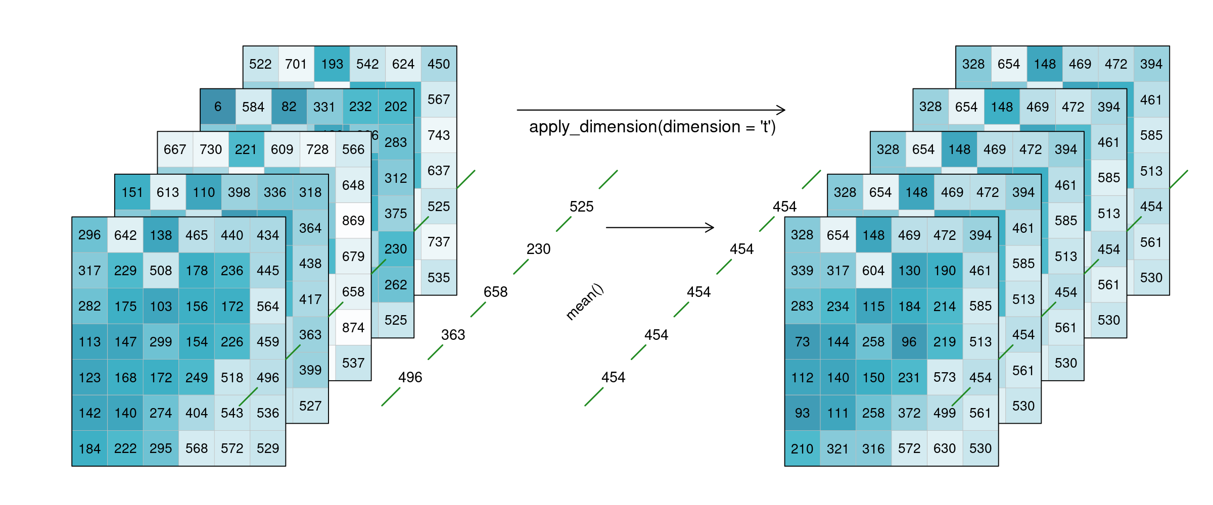
Alternatively, a process can also be applied along a dimension of the datacube, meaning the input is no longer a neighbourhood of some sort but all pixels along that dimension (n equals the complete dimension). If a process is applied along the time dimension (e.g. a breakpoint detection), the complete pixel timeseries are the input. If a process is applied along the spatial dimensions (e.g. a mean), all pixels of an image are the input. The process is then applied to all pixels along that dimension and the dimension continues to exist. This is in contrast to reduce. In the image below, a mean is applied to the time dimension. An example pixel timeseries is highlighted by a green line and processed step-by-step.
# Resample
In a resampling processes (e.g. resample_cube_spatial (opens new window), resample_cube_temporal (opens new window)), the layout of a certain dimension is changed into another layout, most likely also changing the resolution of that dimension. This is done by mapping values of the source (old) datacube to the new layout of the target (new) datacube. During that process, resolutions can be upscaled or downscaled (also called upsampling and downsampling), depending on whether they have a finer or a coarser spacing afterwards. A function is then needed to translate the existing data into the new resolution. A prominent example is to reproject a datacube into the coordinate reference system of another datacube, for example in order to merge the two cubes.
Simplified
resample(🖼️, downscale) => 🟦
resample(🌍, reproject) => 🗺️
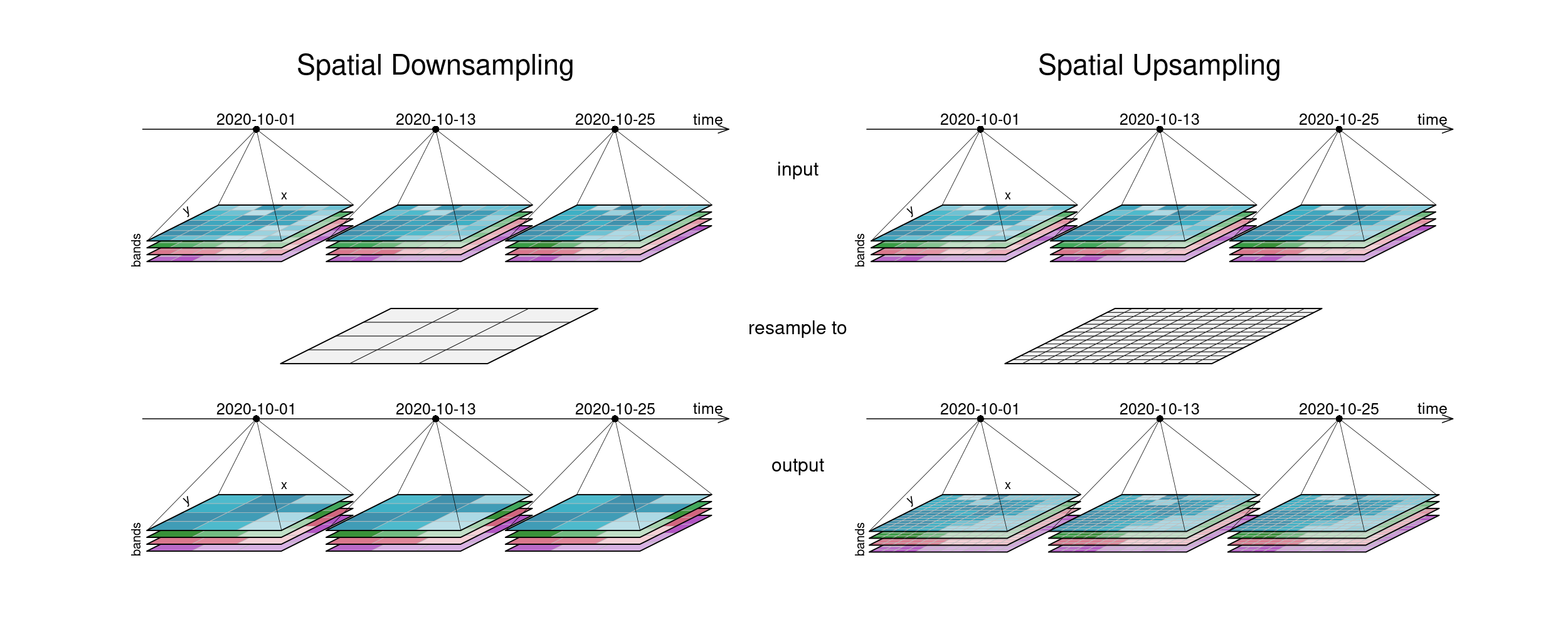
The first figure gives an overview of temporal resampling. How exactly the input timesteps are rescaled to the output timesteps depends on the resampling function.
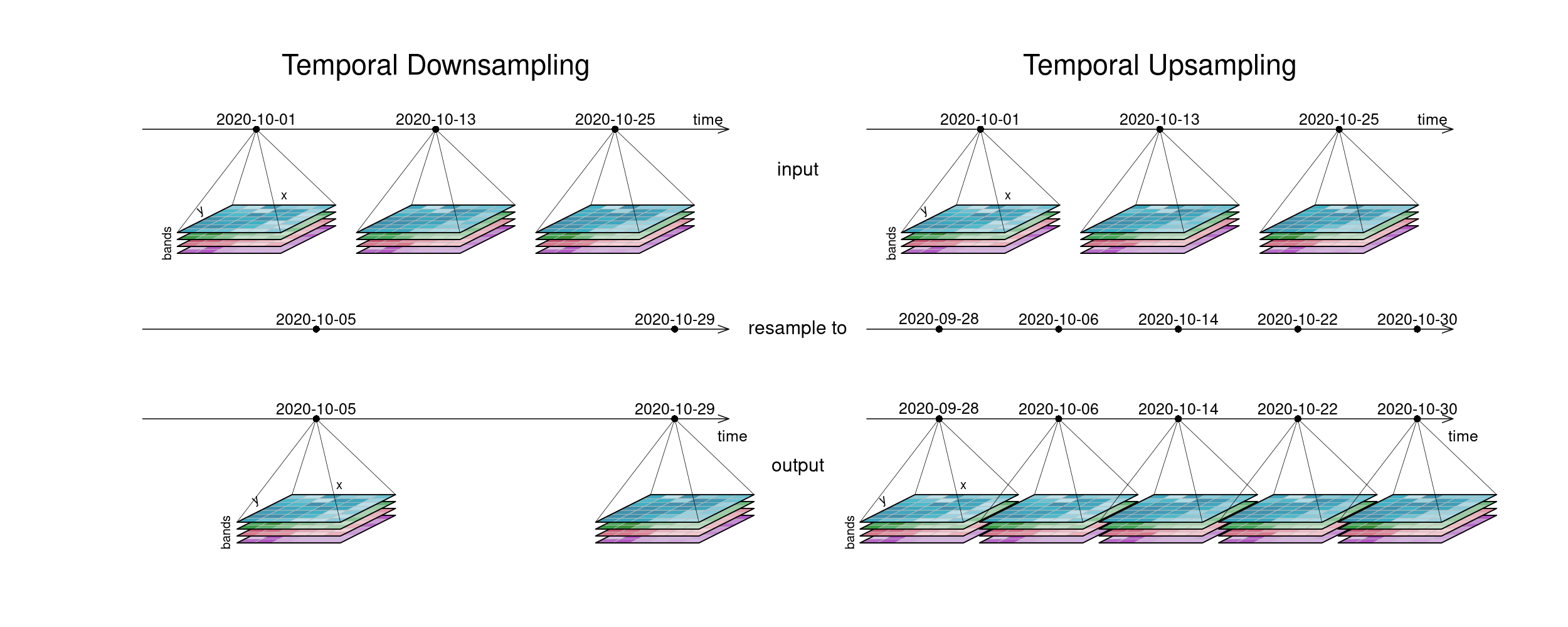
The second figure displays spatial resampling. Observe how in the upsampling process, the output datacube has not gained in information value. The resulting grid still carries the same pixel information, but in higher spatial resolution. Other upsampling methods may yield smoother results, e.g. by using interpolation.
# Reduce
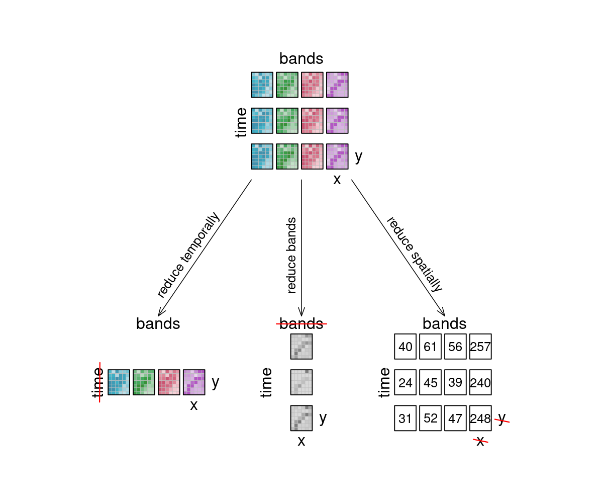
The reduce_dimension (opens new window) process collapses a whole dimension of the datacube. It does so by using some sort of reducer, which is a function that calculates a single result from an amount of values, as e.g. mean(), min() and max() are. For example we can reduce the time dimension (t) of a timeseries by calculating the mean value of all timesteps for each pixel. We are left with a cube that has no time dimension, because all values of that dimension are compressed into a single mean value. The same goes for e.g. the spatial dimensions: If we calculate the mean along the x and y dimensions, we are left without any spatial dimensions, but a mean value for each instance that previously was a raster is returned. In the image below, the dimensions that are reduced are crossed out in the result.
Simplified
reduce([🥬, 🥒, 🍅, 🧅], prepare) => 🥗
Think of it as a waste press that does math instead of using brute force. Given a representation of our example datacube, let's see how it is affected.
# Aggregate
An aggregation of a datacube can be thought of as a grouped reduce. That means it consists of two steps:
- Grouping via a grouping variable, i.e. spatial geometries or temporal intervals
- Reducing these groups along the grouped dimension with a certain reducer function, e.g. calculating the mean pixel value per polygon or the maximum pixel values per month
While the layout of the reduced dimension is changed, other dimensions keep their resolution and geometry. But in contrast to pure reduce, the dimensions along which the reducer function is applied still exist after the operation.
Simplified
aggregate(👪 👩👦 👨👩👦👦, countFamilyMembers) => [3️⃣, 2️⃣, 4️⃣]
A temporal aggregation (e.g. aggregate_temporal (opens new window)) is similar to the downsampling process, as it can be seen in the according image above. Intervals for grouping can either be set manually, or periods can be chosen: monthly, yearly, etc. All timesteps in an interval are then collapsed via a reducer function (mean, max, etc.) and assigned to the given new labels.
A spatial aggregation (e.g. aggregate_spatial (opens new window)) works in a similar manner. Polygons, lines and points can be selected for grouping. Their spatial dimension is then reduced by a given process and thus, a vector cube is returned. The vector cube then has dimensions containing features, attributes and time. In the graphic below, the grouping is only shown for the first timestep.
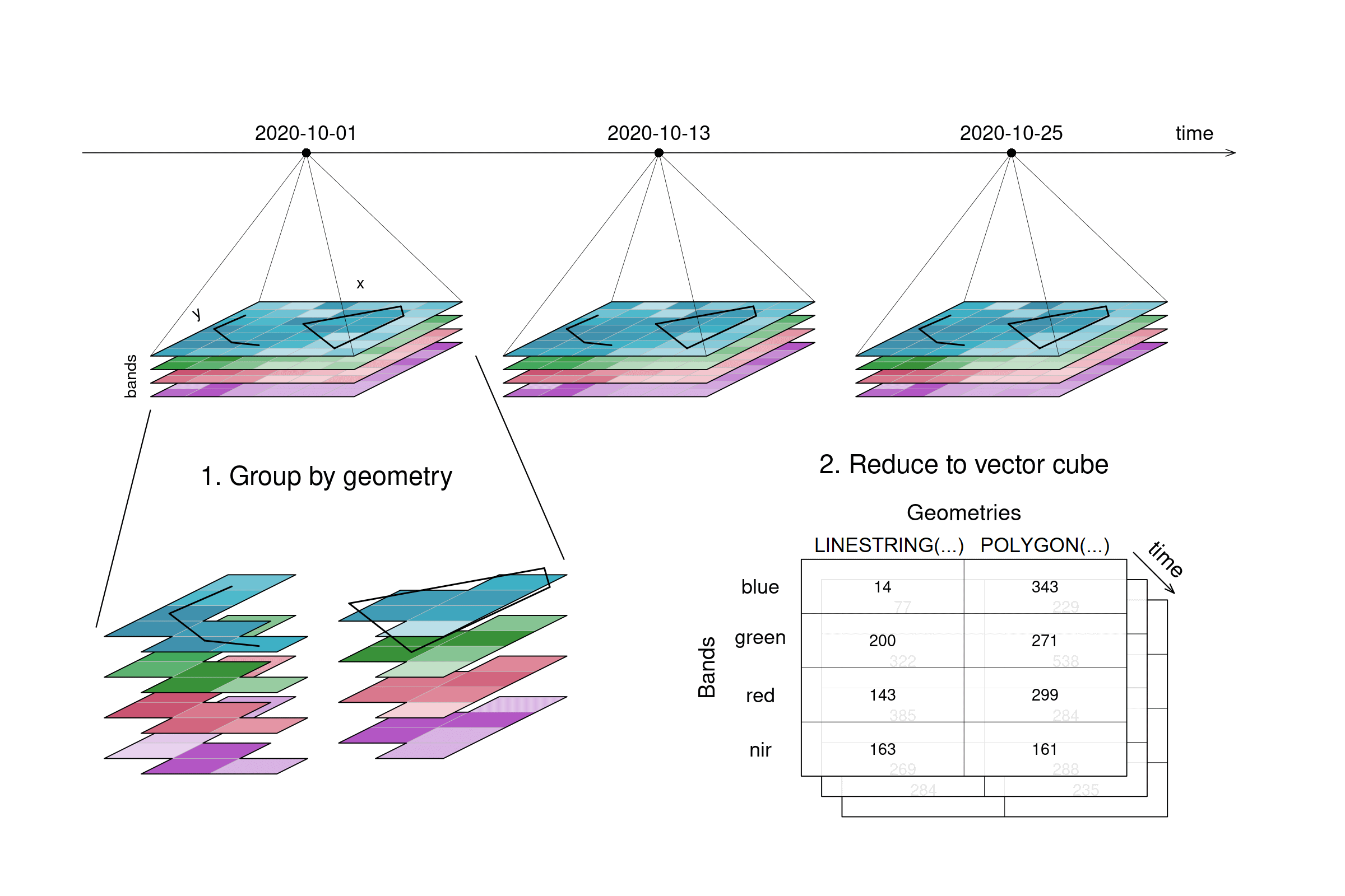
aggregate_spatial specifically can only handle data cubes with three dimensions as of now.