# Python Client

This Getting Started guide will give you just a simple overview of the capabilities of the openEO Python client library. More in-depth information can be found in its official documentation (opens new window).

# Installation

The openEO Python client library is available on PyPI (opens new window) and can easily be installed with a tool like pip, for example:

pip install openeo

The client library is also available on Conda Forge (opens new window).

It's recommended to work in a virtual environment of some kind (venv, conda, ...), containing Python 3.6 or higher.

TIP

For more details, alternative installation procedures or troubleshooting tips: see the official openeo package installation documentation (opens new window).

# Exploring a back-end

If you do not know an openEO back-end that you want to connect to yet, you can have a look at the openEO Hub (opens new window), to find all known back-ends with information on their capabilities.

For this tutorial we will use the openEO instance of Google Earth Engine, which is available at https://earthengine.openeo.org. Note that the code snippets in this guide work the same way for the other back-ends listed in the openEO Hub. Just the collection identifier and band names might differ.

First we need to establish a connection to the back-end.

import openeo

connection = openeo.connect("https://earthengine.openeo.org")

The Connection object (opens new window) is your central gateway to

list data collections, available processes, file formats and other capabilities of the back-end
start building your openEO algorithm from the desired data on the back-end
execute and monitor (batch) jobs on the back-end
etc.

# Collections

The EO data available at a back-end is organised in so-called collections. For example, a back-end might provide fundamental satellite collections like "Sentinel 1" or "Sentinel 2", or preprocessed collections like "NDVI". Collections are used as input data for your openEO jobs.

Note

More information on how openEO "collections" relate to terminology used in other systems can be found in (the openEO glossary).

Let's list all available collections on the back-end, using list_collections (opens new window):

print(connection.list_collections())

which returns list of collection metadata dictionaries, e.g. something like:

[{'id': 'AGERA5', 'title': 'ECMWF AGERA5 meteo dataset', 'description': 'Daily surface meteorolociga datal ...', ...},
 {'id': 'SENTINEL2_L2A_SENTINELHUB', 'title': 'Sentinel-2 top of canopy', ...},
 {'id': 'SENTINEL1_GRD', ...},
 ...]

This listing includes basic metadata for each collection. If necessary, a more detailed metadata listing for a given collection can be obtained with describe_collection (opens new window).

TIP

Programmatically listing collections is just a very simple usage example of the Python client. In reality, you probably want to look up or inspect available collections in a web based overview such as the openEO Hub (opens new window).

# Processes

Processes in openEO are operations that can be applied on (EO) data (e.g. calculate the mean of an array, or mask out observations outside a given polygon). The output of one process can be used as the input of another process, and by doing so, multiple processes can be connected that way in a larger "process graph": a new (user-defined) processes that implements a certain algorithm.

Note

Check the openEO glossary for more details on pre-defined, user-defined processes and process graphs.

Let's list the (pre-defined) processes available on the back-end with list_processes (opens new window):

print(connection.list_processes())

which returns a list of dictionaries describing the process (including expected arguments and return type), e.g.:

[{'id': 'absolute', 'summary': 'Absolute value', 'description': 'Computes the absolute value of a real number `x`, which is th...', 
 {'id': 'mean', 'summary': 'Arithmetic mean(average)', ...}
 ...]

Like with collections, instead of programmatic exploration you'll probably prefer a web-based overview such as the openEO Hub (opens new window) for back-end specific process descriptions or browse the reference specifications of openEO processes (opens new window).

# Authentication

In the code snippets above we did not need to log in since we just queried publicly available back-end information. However, to run non-trivial processing queries one has to authenticate so that permissions, resource usage, etc. can be managed properly.

Depending on the back-end, there might be two different approaches to authenticate. You need to inform yourself at your back-end provider of choice, which authentication approach you have to carry out. You can also have a look at the openEO Hub (opens new window) to see the available authentication types of the back-ends.

A detailed description of why and how to use the authentication methods is on the official documentation (opens new window).

Recommendation

The Google Earth Engine implementation for openEO only supports Basic authentication, but generally the preferred authentication method is OpenID Connect due to better security mechanisms implemented in the OpenID Connect protocol.

# Basic Authentication

The Basic authentication method is a common way of authenticate HTTP requests given username and password.

The following code snippet shows how to log in via Basic authentication:

print("Authenticate with Basic authentication")
connection.authenticate_basic("username", "password")

TIP

You can get username and password here: https://github.com/Open-EO/openeo-earthengine-driver#demo (opens new window)

After successfully calling the authenticate_basic (opens new window) method, you are logged into the back-end with your account.

This means, that every call that comes after that via the connection variable is executed by your user account.

# OpenID Connect Authentication

WARNING

For Google Earth Engine, only Basic Authentication is supported at the moment.

The OIDC (OpenID Connect (opens new window)) authentication can be used to authenticate via an external service given a client ID. The following code snippet shows how to log in via OIDC authentication:

print("Authenticate with OIDC authentication")
connection.authenticate_oidc()

Calling this method opens your system web browser, with which you can authenticate yourself on the back-end authentication system. After that the website will give you the instructions to go back to the python client, where your connection has logged your account in. This means that every call that comes after that via the connection variable is executed by your user account.

# Working with Datacube

Now that we know how to discover the capabilities of the back-end and how to authenticate, let's do some real work and process some EO data in a batch job. We'll build the desired algorithm by working on so-called "Datacubes", which is the central concept in openEO to represent EO data, as discussed in great detail here.

# Creating a Datacube

The first step is loading the desired slice of a data collection with Connection.load_collection (opens new window):

datacube = connection.load_collection(
  "SENTINEL1_GRD",
  spatial_extent={"west": 16.06, "south": 48.06, "east": 16.65, "north": 48.35},
  temporal_extent=["2017-03-01", "2017-04-01"],
  bands=["VV", "VH"]
)

This results in a Datacube object (opens new window) containing the "SENTINEL1_GRD" data restricted to the given spatial extent, the given temporal extend and the given bands .

TIP

You can also filter the datacube step by step or at a later stage by using the following filter methods:

datacube = datacube.filter_bbox(west=16.06, south=48.06, east=16.65, north=48.35)
datacube = datacube.filter_temporal(start_date="2017-03-01", end_date="2017-04-01")
datacube = datacube.filter_bands(["VV", "VH"])

Still, it is recommended to always use the filters directly in load_collection (opens new window) to avoid loading too much data upfront.

# Applying processes

By applying an openEO process on a datacube, we create a new datacube object that represents the manipulated data. The standard way to do this with the Python client is to call the appropriate Datacube object (opens new window) method. The most common or popular openEO processes have a dedicated Datacube method (e.g. mask, aggregate_spatial, filter_bbox, ...). Other processes without a dedicated method can still be applied in a generic way. An on top of that, there are also some convenience methods that implement openEO processes is a compact, Pythonic interface.

For example, the min_time (opens new window) method implements a reduce_dimension process along the temporal dimension, using the min process as reducer function:

datacube = datacube.min_time()

This creates a new datacube (we overwrite the existing variable), where the time dimension is eliminated and for each pixel we just have the minimum value of the corresponding timeseries in the original datacube.

See the Python client Datacube API (opens new window) for a more complete listing of methods that implement openEO processes.

openEO processes that are not supported by a dedicated Datacube method can be applied in a generic way with the process method (opens new window), e.g.:

datacube = datacube.process(
    process_id="ndvi", 
    arguments={
        "data": datacube, 
        "nir": "B8", 
        "red": "B4"}
)

This applies the ndvi process (opens new window) to the datacube with the arguments of "data", "nir" and "red" (This example assumes a datacube with bands B8 and B4).

Note

Still unsure on how to make use of processes with the Python client? Visit the official documentation on working with processes (opens new window).

# Defining output format

After applying all processes you want to execute, we need to tell the back-end to export the datacube, for example as GeoTiff:

result = datacube.save_result("GTiff")

# Execution

It's important to note that all the datacube processes we applied up to this point are not actually executed yet, neither locally nor remotely on the back-end. We just built an abstract representation of the algorithm (input data and processing chain), encapsulated in a local Datacube object (e.g. the result variable above). To trigger an actual execution (on the back-end) we have to explicitly send this representation to the back-end.

openEO defines several processing modes, but for this introduction we'll focus on batch jobs, which is a good default choice.

# Batch job execution

The result datacube object we built above describes the desired input collections, processing steps and output format. We can now just send this description to the back-end to create a batch job with the create_job method (opens new window) like this:

# Creating a new job at the back-end by sending the datacube information.
job = result.create_job()

The batch job, which is referenced by the returned job object, is just created at the back-end, it is not started yet. To start the job and let your Python script wait until the job has finished then download it automatically, you can use the start_and_wait method.

# Starts the job and waits until it finished to download the result.
job.start_and_wait()
job.get_results().download_files("output")

When everything completes successfully, the processing result will be downloaded as a GeoTIFF file in a folder "output".

TIP

The official openEO Python Client documentation has more information on batch job basics (opens new window) or more detailed batch job (result) management (opens new window)

# Full Example

In this chapter we will show a full example of an earth observation use case using the Python client and the Google Earth Engine back-end.

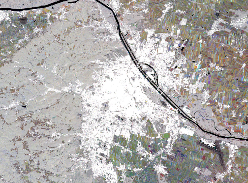
Use Case

We want to produce a monthly RGB composite of Sentinel 1 backscatter data over the area of Vienna, Austria for three months in 2017. This can be used for classification and crop monitoring.

In the following code example, we use inline code comments to describe what we are doing.

WARNING

The username and password in the example above work at the time of writing, but may be invalid at the time you read this. Please contact us for credentials.

import openeo

# First, we connect to the back-end and authenticate ourselves via Basic authentication. 
con = openeo.connect("https://earthengine.openeo.org")
con.authenticate_basic("group11", "test123")

# Now that we are connected, we can initialize our datacube object with the area around Vienna 
# and the time range of interest using Sentinel 1 data.
datacube = con.load_collection("COPERNICUS/S1_GRD",
                               spatial_extent={"west": 16.06, "south": 48.06, "east": 16.65, "north": 48.35},
                               temporal_extent=["2017-03-01", "2017-06-01"],
                               bands=["VV"])

# Since we are creating a monthly RGB composite, we need three (R, G and B) separated time ranges.
# Therefore, we split the datacube into three datacubes by filtering temporal for March, April and May. 
march = datacube.filter_temporal("2017-03-01", "2017-04-01")
april = datacube.filter_temporal("2017-04-01", "2017-05-01")
may = datacube.filter_temporal("2017-05-01", "2017-06-01")

# Now that we split it into the correct time range, we have to aggregate the timeseries values into a single image.
# Therefore, we make use of the Python Client function `mean_time`, which reduces the time dimension, 
# by taking for every timeseries the mean value.

mean_march = march.mean_time()
mean_april = april.mean_time()
mean_may = may.mean_time()

# Now the three images will be combined into the temporal composite. 
# Before merging them into one datacube, we need to rename the bands of the images, because otherwise, 
# they would be overwritten in the merging process.  
# Therefore, we rename the bands of the datacubes using the `rename_labels` process to "R", "G" and "B".
# After that we merge them into the "RGB" datacube, which has now three bands ("R", "G" and "B")

R_band = mean_march.rename_labels(dimension="bands", target=["R"])
G_band = mean_april.rename_labels(dimension="bands", target=["G"])
B_band = mean_may.rename_labels(dimension="bands", target=["B"])

RG = R_band.merge_cubes(G_band)
RGB = RG.merge_cubes(B_band)


# Last but not least, we add the process to save the result of the processing. There we define that 
# the result should be a GeoTiff file.
# We also set, which band should be used for "red", "green" and "blue" color in the options.

RGB = RGB.save_result(format="GTIFF-THUMB")

# With the last process we have finished the datacube definition and can create and start the job at the back-end.

job = RGB.create_job()
job.start_and_wait().download_results()

Now the resulting GTiff file of the RGB backscatter composite is in your current directory.

RGB composite

The source code (opens new window) of this example can be found on GitHub.

# User Defined Functions

If your use case can not be accomplished with the default processes of openEO, you can define a user defined function. Therefore, you can create a Python function that will be executed at the back-end and functions as a process in your process graph.

Detailed information about Python UDFs can be found in the official documentation (opens new window) as well as examples in the Python client repository (opens new window).

# Additional Information

Additional information and resources about the openEO Python Client Library:

Applicable API Versions

Other Page Versions

# Python Client

# Installation

# Exploring a back-end

# Collections

# Processes

# Authentication

# Basic Authentication

# OpenID Connect Authentication

# Working with Datacube

# Creating a Datacube

# Applying processes

# Defining output format

# Execution

# Batch job execution

# Full Example

# User Defined Functions

# Additional Information