# Glossary
This glossary introduces the major technical terms used in the openEO project.
# General terms
- EO: Earth observation
- API: application programming interface (wikipedia (opens new window)); a communication protocol between client and back-end
- client: software tool or environment that end-users directly interact with, e.g. R (RStudio), Python (Jupyter notebook), and JavaScript (web browser); R and Python are two major data science platforms; JavaScript is a major language for web development
- (cloud) back-end: server; computer infrastructure (one or more physical computers or virtual machines) used for storing EO data and processing it
- big Earth observation cloud back-end: server infrastructure where industry and researchers analyse large amounts of EO data
# Processes and process graphs
The terms process and process graph have specific meanings in the openEO API specification.
A process is an operation provided by the back end that performs a specific task on a set of parameters and returns a result. An example is computing a statistical operation, such as mean or median, on selected EO data. A process is similar to a function or method in programming languages.
A process graph chains specific process calls together. Similarly to scripts in the context of programming, process graphs organize and automate the execution of one or more processes that could alternatively be executed individually. In a process graph, processes need to be specific, i.e. concrete values for input parameters need to be specified. These arguments can again be process graphs, scalar values, arrays or objects.
# EO data (Collections)
In our domain, different terms are used to describe EO data(sets). Within openEO, a granule (sometimes also called item or asset in the specification) typically refers to a limited area and a single overpass leading to a very short observation period (seconds) or a temporal aggregation of such data (e.g. for 16-day MODIS composites). A collection is a sequence of granules sharing the same product specification. It typically corresponds to the series of products derived from data acquired by a sensor on board a satellite and having the same mode of operation.
The CEOS OpenSearch Best Practice Document v1.2 (opens new window) lists the following synonyms used by other organizations:
- granule: dataset (ESA, ISO 19115), granule (NASA), product (ESA, CNES), scene (JAXA)
- collection: dataset series (ESA, ISO 19115), collection (CNES, NASA), dataset (JAXA), product (JAXA)
In openEO, a back-end offers a set of collections to be processed. All collections can be requested using a client and are described using the STAC (SpatioTemporal Asset Catalog) metadata specification (opens new window) as STAC collections. A user can load (a subset of) a collection using a special process, which returns a (spatial) data cube. All further processing is then applied to the data cube on the back-end.
# Spatial data cubes
A spatiotemporal data cube is a multidimensional array with one or more spatial or temporal dimensions. In the EO domain, it is common to be implicit about the temporal dimension and just refer to them as spatial data cubes in short. Special cases are raster and vector data cubes.
The figure below shows the data of a four-dimensional (8 x 8 x 2 x 2) raster data cube, with dimension names and values:
| # | dimension name | dimension values |
|---|---|---|
| 1 | x | 288790.5, 288819, 288847.5, 288876, 288904.5, 288933, 288961.5, 288990 |
| 2 | y | 9120747, 9120718, 9120690, 9120661, 9120633, 9120604, 9120576, 9120547 |
| 3 | band | red, green |
| 4 | time | 2018-02-10, 2018-02-17 |
dimensions x and time are aligned along the x-axis; y and band are aligned along the y-axis.
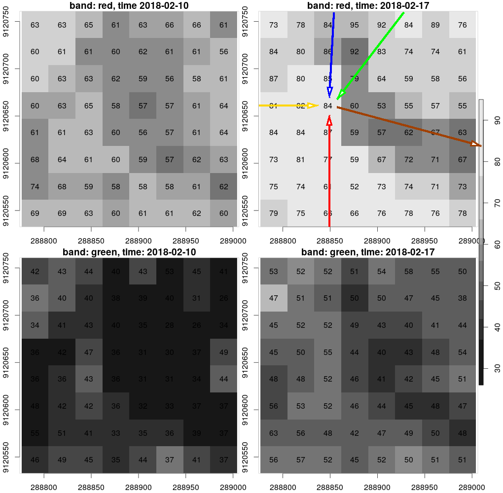
Data cubes as defined here have a single value (scalar) for each unique combination of dimension values. The value pointed to by arrows corresponds to the combination of x=288847.5 (red arrow), y=9120661 (yellow arrow), band=red (blue arrow), time=2018-02-17 (green arrow), and its value is 84 (brown arrow).
If the data concerns grayscale imagery, we could call this single
value a pixel value. One should keep in mind that it is never
a tuple of, say, {red, green, blue} values. "Cell value of a
single raster layer" would be a better analogy; data cube cell
value may be a good compromise.
A data cube stores some additional properties per dimension such as:
- name
- axis / number
- type
- extents or nominal dimension values
- reference systems / projections
- resolutions
Having these properties available allows to easily resample from one data cube to another for example.
# apply: processes that do not change dimensions
Math process that does not reduce or change anything to the array
dimensions. The process apply can be used to apply unary functions
such as abs or sqrt to all values in a data cube.
The process apply_dimension applies (maps) an n-ary function to a particular
dimension. An example along the time dimension is to apply a moving
average filter to implement temporal smoothing.
An example of apply_dimension to the spatial dimensions
is to do a historgram stretch for every spatial (grayscale) image
of an image time series.
# filter: subsetting dimensions by dimension value selection
The filter process makes a cube smaller by selecting specific
value ranges for a particular dimension.
Examples:
- a band filter that selects the
redband - a bounding box filter "crops" the collection to a spatial extent
# reduce: removing dimensions entirely by computation
The reduce process removes a dimension by "rolling up" or summarizing
the values along that dimension to a single value.
For example: eliminate the time dimension by taking the mean along that dimension.
Another example is taking the sum or max along the band dimension.
# aggregate: reducing resolution
Aggregation computes new values from sets of values that are uniquely assigned to groups. It involves a grouping predicate (e.g. monthly, 100 m x 100 m grid cells, or a set of non-overlapping spatial polygons), and an reducer (e.g., mean) that computes one or more new values from the original ones.
In effect, aggregate combines the following three steps:
- split the data cube in groups, based on dimension constraints (time intervals, band groups, spatial polygons)
- apply a reducer to each group (similar to the
reduceprocess, but reducing a group rather than an entire dimension) - combine the result to a new data cube, with some dimensions having reduced resolution (or e.g. raster to vector converted)
Examples:
- a weekly time series may be aggregated to monthly values by computing the
meanfor all values in a month (grouping predicate: months) - spatial aggregation involves computing e.g. mean pixel values on a 100 x 100 m grid, from 10 m x 10 m pixels, where each original pixel is assigned uniquely to a larger pixel (grouping predicate: 100 m x 100 m grid cells)
# resample: changing data cube geometry
Resampling considers the case where we have data at one resolution and coordinate reference system, and need values at another. In case we have values at a 100 m x 100 m grid and need values at a 10 m x 10 m grid, the original values will be reused many times, and may be simply assigned to the nearest high resolution grid cells (nearest neighbor method), or may be interpolated using various methods (e.g. by bilinear interpolation). This is often called upsampling or upscaling.
Resampling from finer to coarser grid is a special case of aggregation often called downsampling or downscaling.
When the target grid or time series has a lower resolution (larger grid cells) or lower frequency (longer time intervals) than the source grid, aggregation might be used for resampling. For example, if the resolutions are similar, (e.g. the source collection provides 10 day intervals and the target needs values for 16 day intervals), then some form of interpolation may be more appropriate than aggregation as defined here.
# User-defined function (UDF)
The abbreviation UDF stands for user-defined function. With this concept, users are able to upload custom code and have it executed e.g. for every pixel of a scene, or applied to a particular dimension or set of dimensions, allowing custom server-side calculations. See the section on UDFs for more information.
# Data Processing modes
Process graphs can be processed in three different ways:
- Results can be pre-computed by creating a batch job using
POST /jobs. They are submitted to the back-end's processing system, but will remain inactive untilPOST /jobs/{job_id}/resultshas been called. They will run only once and store results after execution. Results can be downloaded. Batch jobs are typically time consuming and user interaction is not possible. This is the only mode that allows to get an estimate about time, volume and costs beforehand. - A more dynamic way of processing and accessing data is to create a secondary web service. They allow web-based access using different protocols such as OGC WMS (opens new window) (Open Geospatial Consortium Web Map Service), OGC WCS (opens new window) (Web Coverage Service) or XYZ tiles (opens new window). These protocols usually allow users to change the viewing extent or level of detail (zoom level). Therefore, computations often run on demand so that the requested data is calculated during the request. Back-ends should make sure to cache processed data to avoid additional/high costs and reduce waiting times for the user.
- Process graphs can also be executed on-demand (i.e. synchronously) by sending the process graph to
POST /result. Results are delivered with the request itself and no job is created. Only lightweight computations, for example small previews, should be executed using this approach as timeouts are to be expected for long-polling HTTP requests (opens new window).